3

Am running Excel 2013 on Windows 10 with 16 GB memory.

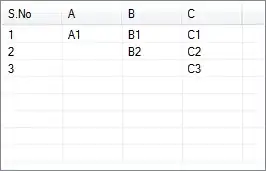
I have a hierarchical structure similar to figure 1 below. My structure is 1000+ rows and as deep as 27 levels.

hierarchy

For a "tree" as depicted above, how to identify the parent of a cell?

Here's what I've done so far. Using conditional formatting, and this formula:

  =AND(A1<>"",OFFSET(A1,1,1)="")

I am able to identify the leaf nodes of the tree, as shown in figure 2 below.

conditional formatting

Now I need to find the immediate ancestor (parent) of every cell (child) in the tree (with the exception of the first row that does not have a parent).

Figure 3 (below) shows an example done manually:

enter image description here

Further, I can associate the tree with an outline. Then I am able to count the number of decimals in the outline in order to track level changes using this formula:

  =LEN(A2)-LEN(SUBSTITUTE(A2,".",""))

as shown in figure 4 below:

enter image description here

How to programmatically accomplish what was done manually in figure 3?

For each row (recorded in a column outside of the tree), print the location of the cell that is the parent of the cell.

Here is a similar question that manually provides "level" information.

How to find parent in an indented hierarchy?

In my case, I need to work from an outline (as shown) or by using a formula for Conditional formatting.
Community
  • 1
  • 1
Jay Gray
  • 1,706
  • 2
  • 20
  • 36
  • Given a `cell`, its parent is `cell.offset(0,-1).end(xlUp)`. – GSerg Jan 01 '17 at 14:29
  • Would you show your solution in a proposed answer? I'm not sure how to apply your comment to my sample? Should I put the sample on a Google Spreadsheet and share the URL? – Jay Gray Jan 01 '17 at 14:32
  • 1
    It's a VBA expression that returns the parent given the cell. I'm not sure how to translate `End(xlUp)` into a formula, it would probably involve a complex, confusing and slow construct. If you're happy with some VBA, create a function that accepts a `c` and returns `c.offset(0,-1).end(xlUp)` and use it from the sheet, otherwise it will probably not help you. – GSerg Jan 01 '17 at 14:37
  • Sounds promising. I had hoped to avoid VBA as I am not a VBA programmer, but will accept it if it works. Would you publish the script so that I can copy/paste into the VBA editor and try it? I would like the values to appear in their own column, either to the left or the right of the hierarchy. – Jay Gray Jan 01 '17 at 14:41
  • Alternatively, if I understand you correctly, I can copy the source to a new tab and apply the VBA to the new (copied) tab. – Jay Gray Jan 01 '17 at 14:48
  • TY. Gimme several hours to apply this to some big hierarchies. BBTY. – Jay Gray Jan 01 '17 at 14:55
  • 2
    I've posted the formula. – GSerg Jan 01 '17 at 15:21

1 Answers1

5

According to your rules, the parent of a cell is the first non-empty cell, bottom to top, in the column immediately to the left:

public function GetParentCell(byval c as range) as range
  set GetParentCell = c.offset(0,-1).end(xlUp)
end function

Having put this in a module, you can use it from the sheet, e.g.

=CELL("address", GetParentCell(D4))

to display the address of the parent of D4.

If you want to avoid VBA completely, you have to find a way to convert End(xlUp) into a formula which may prove difficult because Excel lookups work from top to bottom and you want the other way round. If I was to do that, I would start from Last non-empty cell in a column.

Given that the hierarchy is contained in A1:G19:

  • In H1, put:

    =MATCH("x",$A1:$G1,0)
    
  • In I1, put

    =CELL("address",INDEX(INDEX($A$1:$G$19,1,H1-1):INDEX($A$1:$G$19,ROW(),H1-1),MAX((INDEX($A$1:$G$19,1,H1-1):INDEX($A$1:$G$19,ROW(),H1-1)<>"")*(ROW(INDEX($A$1:$G$19,1,H1-1):INDEX($A$1:$G$19,ROW(),H1-1))))))
    

    as an array formula (CTRL+Shift+Enter).

    The credit goes to https://stackoverflow.com/a/5442955/11683 because it is nothing more than a dynamic version of =INDEX(A:A,MAX((A:A<>"")*(ROW(A:A)))).

  • Drag everything down.

The formula in column I returns the parent of each cell as a true reference which is then examined by the CELL() function to show the address. You can remove the CELL() and use the calculated reference in a different way.

Community
  • 1
  • 1
GSerg
  • 76,472
  • 17
  • 159
  • 346
  • Am I doing this correctly. The H column works correctly. The I column returns the correct column. But the value of the row is always $1. For example, H12 is 7 (column G). But I12 is $F$1, when it should be $F$11. Similarly, H4 is 4 (correct). However I4 is $C$1 but should be $C$3. What am I doing wrong? – Jay Gray Jan 01 '17 at 16:10
  • 2
    You missed the "as an array formula (CTRL+Shift+Enter)", didn't you. – GSerg Jan 01 '17 at 17:42