Last non-empty cell in a column

Question

Does anyone know the formula to find the value of the last non-empty cell in a column, in Microsoft Excel?

Answer 1

Using following simple formula is much faster

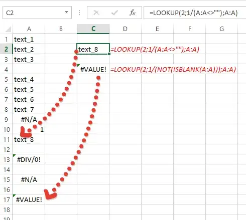
=LOOKUP(2,1/(A:A<>""),A:A)

For Excel 2003:

=LOOKUP(2,1/(A1:A65535<>""),A1:A65535)

It gives you following advantages:

• it's not array formula
• it's not volatile formula

Explanation:

• (A:A<>"") returns array {TRUE,TRUE,..,FALSE,..}
• 1/(A:A<>"") modifies this array to {1,1,..,#DIV/0!,..}.
• Since LOOKUP expects sorted array in ascending order, and taking into account that if the LOOKUP function can not find an exact match, it chooses the largest value in the lookup_range (in our case {1,1,..,#DIV/0!,..}) that is less than or equal to the value (in our case 2), formula finds last 1 in array and returns corresponding value from result_range (third parameter - A:A).

Also little note - above formula doesn't take into account cells with errors (you can see it only if last non empty cell has error). If you want to take them into account, use:

=LOOKUP(2,1/(NOT(ISBLANK(A:A))),A:A)

image below shows the difference:

Answer 2

This works with both text and numbers and doesn't care if there are blank cells, i.e., it will return the last non-blank cell.

It needs to be array-entered, meaning that you press Ctrl-Shift-Enter after you type or paste it in. The below is for column A:

=INDEX(A:A,MAX((A:A<>"")*(ROW(A:A))))

Answer 3

Here is another option: =OFFSET($A$1;COUNTA(A:A)-1;0)

Answer 4

I know this question is old, but I'm not satisfied with the answers provided.

• LOOKUP, VLOOKUP and HLOOKUP has performance issues and should really never be used.

• Array functions has a lot of overhead and can also have performance issues, so it should only be used as a last resort.

• COUNT and COUNTA run into problems if the data is not contiguously non-blank, i.e. you have blank spaces and then data again in the range in question

• INDIRECT is volatile so it should only be used as a last resort

• OFFSET is volatile so it should only be used as a last resort

• any references to the last row or column possible (the 65536th row in Excel 2003, for instance) is not robust and results in extra overhead

This is what I use

• when the data type is mixed: =max(MATCH(1E+306,[RANGE],1),MATCH("*",[RANGE],-1))

• when it's known that the data contains only numbers: =MATCH(1E+306,[RANGE],1)

• when it's known that the data contains only text: =MATCH("*",[RANGE],-1)

MATCH has the lowest overhead and is non-volatile, so if you're working with lots of data this is the best to use.

Answer 5

Inspired by the great lead given by Doug Glancy's answer, I came up with a way to do the same thing without the need of an array-formula. Do not ask me why, but I am keen to avoid the use of array formulae if at all possible (not for any particular reason, it's just my style).

Here it is:

=SUMPRODUCT(MAX(($A:$A<>"")*(ROW(A:A))))

For finding the last non-empty row using Column A as the reference column

=SUMPRODUCT(MAX(($1:$1<>"")*(COLUMN(1:1))))

For finding the last non-empty column using row 1 as the reference row

This can be further utilized in conjunction with the index function to efficiently define dynamic named ranges, but this is something for another post as this is not related to the immediate question addressed herein.

I've tested the above methods with Excel 2010, both "natively" and in "Compatibility Mode" (for older versions of Excel) and they work. Again, with these you do not need to do any of the Ctrl+Shift+Enter. By leveraging the way sumproduct works in Excel we can get our arms around the need to carry array-operations but we do it without an array-formula. I hope someone out there may appreciate the beauty, simplicity and elegance of these proposed sumproduct solutions as much as I do. I do not attest to the memory-efficiency of the above solutions though. Just that they are simple, look beautiful, help the intended purpose and are flexible enough to extend their use to other purposes :)

Hope this helps!

All the best!

Answer 6

This works in Excel 2003 (& later with minor edit, see below). Press Ctrl+Shift+Enter (not just Enter) to enter this as an array formula.

=IF(ISBLANK(A65536),INDEX(A1:A65535,MAX((A1:A65535<>"")*(ROW(A1:A65535)))),A65536)

Be aware that Excel 2003 is unable to apply an array formula to an entire column. Doing so yields #NUM!; unpredictable results may occur! (EDIT: Conflicting information from Microsoft: The same may or may not be true about Excel 2007; problem may have been fixed in 2010.)

That's why I apply the array formula to range A1:A65535 and give special treatment to the last cell, which is A65536 in Excel 2003. Can't just say A:A or even A1:A65536 as the latter automatically reverts to A:A.

If you're absolutely sure A65536 is blank, then you can skip the IF part:

=INDEX(A1:A65535,MAX((A1:A65535<>"")*(ROW(A1:A65535))))

Note that if you're using Excel 2007 or 2010, the last row number is 1048576 not 65536, so adjust the above as appropriate.

If there are no blank cells in the middle of your data, then I would just use the simpler formula, =INDEX(A:A,COUNTA(A:A)).

Answer 7

An alternative solution without array formulas, possibly more robust than that of a previous answer with a (hint to a) solution without array formulas, is

=INDEX(A:A,INDEX(MAX(($A:$A<>"")*(ROW(A:A))),0))

See this answer as an example. Kudos to Brad and barry houdini, who helped solving this question.

Possible reasons for preferring a non-array formula are given in:

1. An official Microsoft page (look for "Disadvantages of using array formulas").
   Array formulas can seem magical, but they also have some disadvantages:

   • You may occasionally forget to press CTRL+SHIFT+ENTER. Remember to press this key combination whenever you enter or edit an array formula.
   • Other users may not understand your formulas. Array formulas are relatively undocumented, so if other people need to modify your workbooks, you should either avoid array formulas or make sure those users understand how to change them.
   • Depending on the processing speed and memory of your computer, large array formulas can slow down calculations.

2. Array Formula Heresy.

Answer 8

if you search in Column (A) use :

=INDIRECT("A" & SUMPRODUCT(MAX((A:A<>"")*(ROW(A:A)))))

if your range is A1:A10 you can use:

=INDIRECT("A" & SUMPRODUCT(MAX(($A$1:$A10<>"")*(ROW($A$1:$A10)))))

in this formula :

SUMPRODUCT(MAX(($A$1:$A10<>"")*(ROW($A$1:$A10))))

returns last non blank row number ,and indirect() returns cell value.

Answer 9

=INDEX(A:A, COUNTA(A:A), 1) taken from here

Answer 10

=MATCH("*";A1:A10;-1) for textual data

=MATCH(0;A1:A10;-1) for numerical data

Answer 11

Ive tried all the non-volatile versions but Not one version given above has worked.. excel 2003/2007update. Surely this can be done in excel 2003. Not as an array nor standard formula. I either get just a blank, 0 or #value error. So I resort to the volatile methods .. This worked..

=LOOKUP(2,1/(T4:T369<>""),T4:T369)

@Julian Kroné .. Using ";" instead of "," does NOT work! I think you are using Libre Office not MS excel? LOOKUP is so annoyingly volitile I use it as a last resort only

Answer 12

For Microsoft office 2013

"Last but one" of a non empty row:

=OFFSET(Sheet5!$C$1,COUNTA(Sheet5!$C:$C)-2,0)

"Last" non empty row:

=OFFSET(Sheet5!$C$1,COUNTA(Sheet5!$C:$C)-1,0)

Answer 13

Microsoft 365:

=XLOOKUP(FALSE,ISBLANK(A:A),A:A,"",,-1)

Answer 14

Place this code in a VBA module. Save. Under functions, User defined look for This function.

Function LastNonBlankCell(Range As Excel.Range) As Variant
    Application.Volatile
    LastNonBlankCell = Range.End(xlDown).Value
End Function

Answer 15

I used HLOOKUP

A1 has a date; A2:A8 has forecasts captured at different times, I want the latest

=Hlookup(a1,a1:a8,count(a2:a8)+1)

This uses a standard hlookup formula with the lookup array defined by the number of entries.

Answer 16

for textual data:

EQUIV("";A1:A10;-1)

for numerical data:

EQUIV(0;A1:A10;-1)

This give you the relative index of the last non empty cell in the range selected (here A1:A10).

If you want to get the value, access it via INDIRECT after building -textually- the absolute cell reference, eg:

INDIRECT("A" & (nb_line_where_your_data_start + EQUIV(...) - 1))

Answer 17

I had the same problem too. This formula also works equally well:-

=INDIRECT(CONCATENATE("$G$",(14+(COUNTA($G$14:$G$65535)-1))))

14 being the row number of the first row in the rows you want to count.

Chronic Clawtooth

Answer 18

If you know that there are not going to be empty cells in between, the fastest way is this.

=INDIRECT("O"&(COUNT(O:O,"<>""")))

It just counts the non-empty cells and refers to the appropriate cell.

It can be used for a specific range as well.

=INDIRECT("O"&(COUNT(O4:O34,"<>""")+3))

This returns the last non empty cell in the range O4:O34.

Answer 19

This formula worked with me for office 2010:

=LOOKUP(2;1/(A1:A100<>"");A1:A100)

A1: the first cell A100: refer to the last cell in comparing

Answer 20

I think the response from W5ALIVE is closest to what I use to find the last row of data in a column. Assuming I am looking for the last row with data in Column A, though, I would use the following for the more generic lookup:

=MAX(IFERROR(MATCH("*",A:A,-1),0),IFERROR(MATCH(9.99999999999999E+307,A:A,1),0))

The first MATCH will find the last text cell and the second MATCH finds the last numeric cell. The IFERROR function returns zero if the first MATCH finds all numeric cells or if the second match finds all text cells.

Basically this is a slight variation of W5ALIVE's mixed text and number solution.

In testing the timing, this was significantly quicker than the equivalent LOOKUP variations.

To return the actual value of that last cell, I prefer to use indirect cell referencing like this:

=INDIRECT("A"&MAX(IFERROR(MATCH("*",A:A,-1),0),IFERROR(MATCH(9.99999999999999E+307,A:A,1),0)))

The method offered by sancho.s is perhaps a cleaner option, but I would modify the portion that finds the row number to this:

=INDEX(MAX((A:A<>"")*(ROW(A:A))),1)

the only difference being that the ",1" returns the first value while the ",0" returns the entire array of values (all but one of which are not needed). I still tend to prefer addressing the cell to the index function there, in other words, returning the cell value with:

=INDIRECT("A"&INDEX(MAX((A:A<>"")*(ROW(A:A))),1))

Great thread!

Answer 21

If you are not afraid to use arrays, then the following is a very simple formula to solve the problem:

=SUM(IF(A:A<>"",1,0))

You must press CTRL + SHIFT + ENTER because this is an array formula.

Answer 22

INDEX returns a value by index position in an array and ROWS then is used to specify the last position of the array.

=LET(array,A1:A10,INDEX(array,ROWS(array)))

Also works for multiple columns when setting the parameter [column_num] of INDEX to 0:

=LET(array,A1:C10,INDEX(array,ROWS(array),0))

Answer 23

We will use a combination of INDEX, MAX, COUNTA, and OFFSET functions.

Assuming you want to find the last non-empty value in column A, use the following formula:

=INDEX(A:A, MAX(ROW(A:A)*(A:A<>"")))

(A:A<>""): This creates an array of TRUE/FALSE values, where TRUE represents non-empty cells in column A.

ROW(A:A)*(A:A<>""): This multiplies the row numbers by the TRUE/FALSE array, giving an array of row numbers for non-empty cells and 0 for empty cells.

MAX(ROW(A:A)*(A:A<>"")): This finds the maximum row number from the array of row numbers, which corresponds to the last non-empty cell in column A.

INDEX(A:A, MAX(ROW(A:A)*(A:A<>""))): Finally, the INDEX function returns the value of the last non-empty cell in column A based on the maximum row number.

Make sure to adjust the column reference in the formula to match your actual data column. Replace all instances of "A:A" with the correct column letter (e.g., "B:B" for column B, "C:C" for column C, and so on).

Please try this formula, and it should give you the value of the last non-empty cell in the specified column. If it still doesn't work, please ensure that your data is contiguous (no empty rows within the range) and that you have data in the specified column.

Answer 24

A simple one which works for me:

=F7-INDEX(A:A,COUNT(A:A))

Answer 25

Okay, so I had the same issue as the asker, and tried both top answers. But only getting formula errors. Turned out that I needed to exchange the "," to ";" for the formulas to work. I am using XL 2007.

Example:

=LOOKUP(2;1/(A:A<>"");A:A)

or

=INDEX(A:A;MAX((A:A<>"")*(ROW(A:A))))

Answer 26

For version tracking (adding the letter v to the beginning of the number), I found this one to work well in Xcelsius (SAP Dashboards)

="v"&MAX(A2:A500)