Consistent size for GraphPlots

Question

Update 10/27: I've put detailed steps for achieving consistent scale in an answer. Basically for each Graphics object you need to fix all padding/margins to 0 and manually specify plotRange and imageSize that such that 1) plotRange includes all graphics 2) imageSize=scale*plotRange

Still now sure how to do 1) in full generality, a solution that works for Graphics consisting of points and thick lines (AbsoluteThickness) is given

---

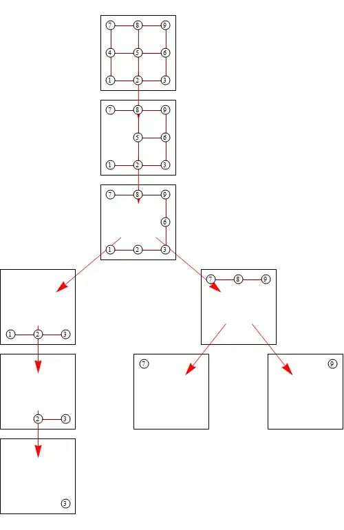
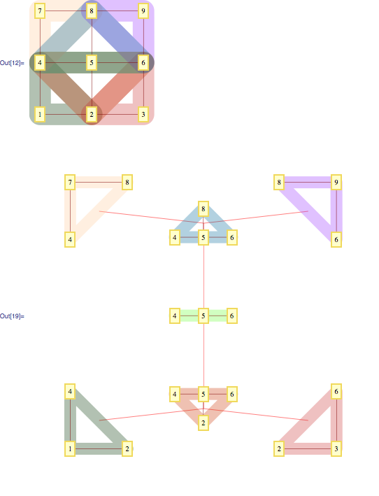
I'm using "Inset" in VertexRenderingFunction and "VertexCoordinates" to guarantee consistent appearance among subgraphs of a graph. Those subgraphs are drawn as vertices of another graph, using "Inset". There are two problems, one is that resulting boxes are not cropped around the graph (ie, graph with one vertex still gets placed in a big box), and another is that there's strange variation among sizes (you can see one box is vertical). Can anyone see a way around these problems?

This is related to an earlier question of how to keep vertex sizes looking the same, and while Michael Pilat's suggestion of using Inset works to keep vertices rendering at the same scale, overall scale may be different. For instance on the left branch, the graph consisting of vertices 2,3 is stretched relative to the "2,3" subgraph in the top graph, even though I'm using absolute vertex positioning for both

_{(source: yaroslavvb.com)}

(*utilities*)intersect[a_, b_] := Select[a, MemberQ[b, #] &];
induced[s_] := Select[edges, #~intersect~s == # &];
Needs["GraphUtilities`"];
subgraphs[
   verts_] := (gr = 
    Rule @@@ Select[edges, (Intersection[#, verts] == #) &];
   Sort /@ WeakComponents[gr~Join~(# -> # & /@ verts)]);

(*graph*)
gname = {"Grid", {3, 3}};
edges = GraphData[gname, "EdgeIndices"];
nodes = Union[Flatten[edges]];
AppendTo[edges, #] & /@ ({#, #} & /@ nodes);
vcoords = Thread[nodes -> GraphData[gname, "VertexCoordinates"]];

(*decompose*)
edgesOuter = {};
pr[_, _, {}] := None;
pr[root_, elim_, 
   remain_] := (If[root != {}, AppendTo[edgesOuter, root -> remain]];
   pr[remain, intersect[Rest[elim], #], #] & /@ 
    subgraphs[Complement[remain, {First[elim]}]];);
pr[{}, {4, 5, 6, 1, 8, 2, 3, 7, 9}, nodes];

(*visualize*)

vrfInner = 
  Inset[Graphics[{White, EdgeForm[Black], Disk[{0, 0}, .05], Black, 
      Text[#2, {0, 0}]}, ImageSize -> 15], #] &;
vrfOuter = 
  Inset[GraphPlot[Rule @@@ induced[#2], 
     VertexRenderingFunction -> vrfInner, 
     VertexCoordinateRules -> vcoords, SelfLoopStyle -> None, 
     Frame -> True, ImageSize -> 100], #] &;
TreePlot[edgesOuter, Automatic, nodes, 
 EdgeRenderingFunction -> ({Red, Arrow[#1, 0.2]} &), 
 VertexRenderingFunction -> vrfOuter, ImageSize -> 500]

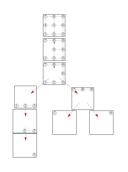
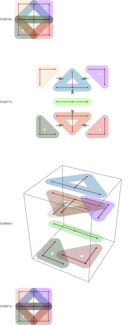
Here's another example, same problem as before, but the difference in relative scales is more visible. The goal is to have parts in the second picture match precisely the parts in the first picture.

_{(source: yaroslavvb.com)}

(* Visualize tree decomposition of a 3x3 grid *)

inducedGraph[set_] := Select[edges, # \[Subset] set &];
Subset[a_, b_] := (a \[Intersection] b == a);
graphName = {"Grid", {3, 3}};
edges = GraphData[graphName, "EdgeIndices"];
vars = Range[GraphData[graphName, "VertexCount"]];
vcoords = Thread[vars -> GraphData[graphName, "VertexCoordinates"]];

plotHighlight[verts_, color_] := Module[{vpos, coords},
   vpos = 
    Position[Range[GraphData[graphName, "VertexCount"]], 
     Alternatives @@ verts];
   coords = Extract[GraphData[graphName, "VertexCoordinates"], vpos];
   If[coords != {}, AppendTo[coords, First[coords] + .002]];
   Graphics[{color, CapForm["Round"], JoinForm["Round"], 
     Thickness[.2], Opacity[.3], Line[coords]}]];

jedges = {{{1, 2, 4}, {2, 4, 5, 6}}, {{2, 3, 6}, {2, 4, 5, 6}}, {{4, 
     5, 6}, {2, 4, 5, 6}}, {{4, 5, 6}, {4, 5, 6, 8}}, {{4, 7, 8}, {4, 
     5, 6, 8}}, {{6, 8, 9}, {4, 5, 6, 8}}};
jnodes = Union[Flatten[jedges, 1]];

SeedRandom[1]; colors = 
 RandomChoice[ColorData["WebSafe", "ColorList"], Length[jnodes]];
bags = MapIndexed[plotHighlight[#, bc[#] = colors[[First[#2]]]] &, 
   jnodes];
Show[bags~
  Join~{GraphPlot[Rule @@@ edges, VertexCoordinateRules -> vcoords, 
    VertexLabeling -> True]}, ImageSize -> Small]

bagCentroid[bag_] := Mean[bag /. vcoords];
findExtremeBag[vec_] := (
   vertList = First /@ vcoords;
   coordList = Last /@ vcoords;
   extremePos = 
    First[Ordering[jnodes, 1, 
      bagCentroid[#1].vec > bagCentroid[#2].vec &]];
   jnodes[[extremePos]]
   );

extremeDirs = {{1, 1}, {1, -1}, {-1, 1}, {-1, -1}};
extremeBags = findExtremeBag /@ extremeDirs;
extremePoses = bagCentroid /@ extremeBags;
vrfOuter = 
  Inset[Show[plotHighlight[#2, bc[#2]], 
     GraphPlot[Rule @@@ inducedGraph[#2], 
      VertexCoordinateRules -> vcoords, SelfLoopStyle -> None, 
      VertexLabeling -> True], ImageSize -> 100], #] &;

GraphPlot[Rule @@@ jedges, VertexRenderingFunction -> vrfOuter, 
 EdgeRenderingFunction -> ({Red, Arrowheads[0], Arrow[#1, 0]} &), 
 ImageSize -> 500, 
 VertexCoordinateRules -> Thread[Thread[extremeBags -> extremePoses]]]

Any other suggestions for aesthetically pleasing visualization of graph operations are welcome.

Answer 1

Here are the steps needed to achieve precise control over relative scales of graphics objects.

To achieve consistent scale one needs to explicitly specify input coordinate range (regular coordinates) and output coordinate range (absolute coordinates). Regular coordinate range depends on PlotRange, PlotRangePadding (and possibly others options?). Absolute coordinate range depends on ImageSize,ImagePadding (and possibly other options?). For GraphPlot, it is sufficient to specify PlotRange and ImageSize.

To create Graphics object that renders at a pre-determined scale, you need to figure out PlotRange needed to fully include the object, corresponding ImageSize and return Graphics object with these settings specified. To figure out the necessary PlotRange when thick lines are involved it is easier to deal with AbsoluteThickness, call it abs. To fully include those lines you could take the smallest PlotRange that includes endpoints, then offset minimum x and maximum y boundaries by abs/2, and offset maximum x and minimum y boundaries by (abs/2+1). Note that these are output coordinates.

When combining several scale-calibrated Graphics objects you need to recalculate PlotRange/ImageSize and set them explicitly for the combined Graphics object.

To Inset scale-calibrated objects into GraphPlot you need to make sure that coordinates used for automatic GraphPlot positioning are in the same range. For that, you could pick several corner nodes, fix their positions manually, and let automatic positioning do the rest.

Primitives Line/JoinedCurve/FilledCurve render joins/caps differently depending on whether the line is (almost) collinear, so one needs to manually detect collinearity.

Using this approach, rendered images should have width equal to

(inputPlotRange*scale + 1) + lineThickness*scale + 1

First extra 1 is to avoid the "fencepost error" and second extra 1 is the extra pixel needed to add on the right to make sure thick lines are not cut-off

I've verified this formula by doing Rasterize on combined Show and rasterizing a 3D plot with objects mapped using Texture and viewed with Orthographic projection and it matches the predicted result. Doing 'Copy/Paste' on objects Inset into GraphPlot, and then Rasterizing, I get an image that's one pixel thinner than predicted.

_{(source: yaroslavvb.com)}

(**** Note, this uses JoinedCurve and Texture which are Mathematica 8 primitives.
      In Mathematica 7, JoinedCurve is not needed and can be removed *)

(** Global variables **)
scale = 50;
lineThickness = 1/2; (* line thickness in regular coordinates *)

(** Global utilities **)

(* test if 3 points are collinear, needed to work around difference \
in how colinear Line endpoints are rendered *)

collinear[points_] := 
 Length[points] == 3 && (Det[Transpose[points]~Append~{1, 1, 1}] == 0)

(* tales list of point coordinates, returns plotRange bounding box, \
uses global "scale" and "lineThickness" to get bounding box *)

getPlotRange[lst_] := (
   {xs, ys} = Transpose[lst];
   (* two extra 1/
   scale offsets needed for exact match *)
   {{Min[xs] - 
      lineThickness/2, 
     Max[xs] + lineThickness/2 + 1/scale}, {Min[ys] - 
      lineThickness/2 - 1/scale, Max[ys] + lineThickness/2}}
   );

(* Gets image size for given plot range *)

getImageSize[{{xmin_, xmax_}, {ymin_, ymax_}}] := (
   imsize = scale*{xmax - xmin, ymax - ymin} + {1, 1}
   );

(* converts plot range to vertices of rectangle *)

pr2verts[{{xmin_, xmax_}, {ymin_, ymax_}}] := {{xmin, ymin}, {xmax, 
    ymin}, {xmax, ymax}, {xmin, ymax}};

(* lifts two dimensional coordinates into 3d *)

lift[h_, coords_] := Append[#, h] & /@ coords
(* convert Raster object to array specification of texture *)

raster2texture[raster_] := Reverse[raster[[1, 1]]/255]

Subset[a_, b_] := (a \[Intersection] b == a);
inducedGraph[set_] := Select[edges, # \[Subset] set &];
values[dict_] := Map[#[[-1]] &, DownValues[dict]];


(** Graph Specific Stuff *)
graphName = {"Grid", {3, 3}};
verts = Range[GraphData[graphName, "VertexCount"]];
edges = GraphData[graphName, "EdgeIndices"];
vcoords = Thread[verts -> GraphData[graphName, "VertexCoordinates"]];
jedges = {{{1, 2, 4}, {2, 4, 5, 6}}, {{2, 3, 6}, {2, 4, 5, 6}}, {{4, 
     5, 6}, {2, 4, 5, 6}}, {{4, 5, 6}, {4, 5, 6, 8}}, {{4, 7, 8}, {4, 
     5, 6, 8}}, {{6, 8, 9}, {4, 5, 6, 8}}};
jnodes = Union[Flatten[jedges, 1]];


(* Generate diagram with explicit PlotRange,ImageSize and \
AbsoluteThickness *)
plotHL[verts_, color_] := (
   coords = verts /. vcoords;
   obj = JoinedCurve[Line[coords], 
     CurveClosed -> Not[collinear[coords]]];

   (* Figure out PlotRange and ImageSize needed to respect scale *)

    pr = getPlotRange[verts /. vcoords];
   {{xmin, xmax}, {ymin, ymax}} = pr;
   imsize = scale*{xmax - xmin, ymax - ymin};
   lineForm = {Opacity[.3], color, JoinForm["Round"], 
     CapForm["Round"], AbsoluteThickness[scale*lineThickness]};
   g = Graphics[{Directive[lineForm], obj}];
   gg = GraphPlot[Rule @@@ inducedGraph[verts], 
     VertexCoordinateRules -> vcoords];
   Show[g, gg, PlotRange -> pr, ImageSize -> imsize]
   );

(* Initialize all graph plot images *)
SeedRandom[1]; colors = 
 RandomChoice[ColorData["WebSafe", "ColorList"], Length[jnodes]];
Clear[bags];
MapThread[(bags[#1] = plotHL[#1, #2]) &, {jnodes, colors}];

(** Ploting parent graph of subgraphs **)

(* figure out coordinates of subgraphs close to edges of bounding \
box, use them to anchor parent GraphPlot *)

bagCentroid[bag_] := Mean[bag /. vcoords];
findExtremeBag[vec_] := (vertList = First /@ vcoords;
   coordList = Last /@ vcoords;
   extremePos = 
    First[Ordering[jnodes, 1, 
      bagCentroid[#1].vec > bagCentroid[#2].vec &]];
   jnodes[[extremePos]]);

extremeDirs = {{1, 1}, {1, -1}, {-1, 1}, {-1, -1}};
extremeBags = findExtremeBag /@ extremeDirs;
extremePoses = bagCentroid /@ extremeBags;

(* figure out new plot range needed to contain all objects *)

fullPR = getPlotRange[verts /. vcoords];
fullIS = getImageSize[fullPR];

(*** Show bags together merged ***)
image1 = 
 Show[values[bags], PlotRange -> fullPR, ImageSize -> fullIS]

(*** Show bags as vertices of another GraphPlot ***)
GraphPlot[
 Rule @@@ jedges,
 EdgeRenderingFunction -> ({Gray, Thick, Arrowheads[.05], 
     Arrow[#1, 0.22]} &),
 VertexCoordinateRules -> 
  Thread[Thread[extremeBags -> extremePoses]],
 VertexRenderingFunction -> (Inset[bags[#2], #] &),
 PlotRange -> fullPR,
 ImageSize -> 3*fullIS
 ]

(*** Show bags as 3d slides ***)
makeSlide[graphics_, pr_, h_] := (
  Graphics3D[{
    Texture[raster2texture[Rasterize[graphics, Background -> None]]],
    EdgeForm[None],
    Polygon[lift[h, pr2verts[pr]], 
     VertexTextureCoordinates -> pr2verts[{{0, 1}, {0, 1}}]]
    }]
  )
yoffset = 1/2;
slides = MapIndexed[
   makeSlide[bags[#], getPlotRange[# /. vcoords], 
     yoffset*First[#2]] &, jnodes];
Show[slides, ImageSize -> 3*fullIS]

(*** Show 3d slides in orthographic projection ***)
image2 = 
 Show[slides, ViewPoint -> {0, 0, Infinity}, ImageSize -> fullIS, 
  Boxed -> False]

(*** Check that 3d and 2d images rasterize to identical resolution ***)
Dimensions[Rasterize[image1][[1, 1]]] == 
 Dimensions[Rasterize[image2][[1, 1]]]

Answer 2

OK, in your comment to my previous answer (this is a different approach), you said the problem was the interaction between GraphPlot/Inset/PlotRange. If you don't specify a size for Inset, then it inherits its size from the ImageSize of the inset Graphics object.

Here's my edit of the final section in you first example, this time taking into account the size of the Inset graphs.

(*visualize*)
vrfInner = Inset[Graphics[{White, EdgeForm[Black], Disk[{0, 0}, .05], Black, 
      Text[#2, {0, 0}]}, ImageSize -> 15], #, Center] &;
vrfOuter = Module[{edges = Rule @@@ induced[#2], prange, psize},
    prange = Union /@ Transpose[Union[Flatten[List @@@ edges]] /. vcoords];
    prange = {Min[#] - .5, Max[#] + .5} & /@ prange;
    psize = Subtract @@@ Reverse /@ prange;
    Inset[GraphPlot[edges, VertexRenderingFunction -> vrfInner, 
       VertexCoordinateRules -> vcoords, SelfLoopStyle -> None, 
       Frame -> True, ImageSize -> 100, PlotRange -> prange, 
       PlotRangePadding -> None], #, Center, Scaled[psize {.05, .04}],
       Background -> None ]] &;
TreePlot[edgesOuter, Automatic, nodes, 
 EdgeRenderingFunction -> ({Red, Arrow[#1, 0.25]} &), 
 VertexRenderingFunction -> vrfOuter, ImageSize -> 500]

n.b. the {.05, .04} would have to be modified as the size and layout of the outer graph changes... To automate the whole thing, you might need a nice way for the inner and outer graphics objects to inspect each other...

Answer 3

You can fix your first example by changing vrfOuter as follows:

vrfOuter =
  Inset[
    Framed@GraphPlot[
      Rule@@@induced[#2],
      VertexRenderingFunction -> vrfInner,
      VertexCoordinateRules -> vcoords,
      SelfLoopStyle -> None,
      ImageSize -> {100, 100},
      AspectRatio -> 1,
      PlotRange -> {{1, 3}, {1, 3}}
    ],
    #
  ] &;

I removed the Frame->All option and added a wrapping call to Framed. This is because I find that I cannot adequately control the margins outside of the frame generated by the former. I might be missing some option somewhere, but Framed works the way I want without fuss.

I added an explicit height to the ImageSize option. Without it, Mathematica tries to choose a height using some algorithm that mostly produces pleasing results, but sometimes (as here) gets confused.

I added the AspectRatio option for the same reason -- Mathematica tries to choose a "pleasing" aspect ratio (typically the Golden Ratio), but we don't want that here.

I added the PlotRange option to ensure that each subgraph is using the same co-ordinate system. Without it, Mathematica will usually select a minimal range that shows all nodes.

The results are shown below. I leave it as an exercise to the reader to adjust the arrows, margins, etc. ;)

Edit: added the PlotRange option in response to a comment by @Yaroslav Bulatov

Answer 4

As a quick hack, you could introduce a ghost graph to force all subgraphs to display on the same grid. Here's my modification of the last part of your first example -- my ghost graph is a copy of your original graph, but with the vertex numbers made negative.

(*visualize*)

ghost = GraphData[gname, "EdgeRules"] /. HoldPattern[a_ -> b_] :> -a -> -b;
vrfInner = If[#2 > 0, 
    Inset[Graphics[{White, EdgeForm[Black], Disk[{0, 0}, .05], Black, 
       Text[#2, {0, 0}]}, ImageSize -> 15], #], {}] &;
erfInner = {If[TrueQ[#2[[1]] > 0], Blue, White], Line[#1]} &;
vrfOuter = Inset[GraphPlot[Join[Rule @@@ induced[#2], ghost],
     VertexRenderingFunction -> vrfInner, 
     VertexCoordinateRules -> (Join[#,#/.HoldPattern[a_->b_]:>-a -> b]&[vcoords]), 
     EdgeRenderingFunction -> erfInner, SelfLoopStyle -> None, 
     Frame -> True, ImageSize -> 100], #] &;
TreePlot[edgesOuter, Automatic, nodes, 
 EdgeRenderingFunction -> ({Red, Arrow[#1, 0.2]} &), 
 VertexRenderingFunction -> vrfOuter, ImageSize -> 500]

You could do the same thing for your second example. Also, if you don't want the wasted vertical space you could write a quick function that checks which nodes are to be displayed and only keeps the ghosts on the needed rows.

Edit: The same output can be obtained by simply setting PlotRange -> {{1, 3}, {1, 3}} for the inner graphs...