How can I efficiently process a numpy array in blocks similar to Matlab's blkproc (blockproc) function

Question

I'm looking for a good approach for efficiently dividing an image into small regions, processing each region separately, and then re-assembling the results from each process into a single processed image. Matlab had a tool for this called blkproc (replaced by blockproc in newer versions of Matlab).

In an ideal world, the function or class would support overlap between the divisions in the input matrix too. In the Matlab help, blkproc is defined as:

B = blkproc(A,[m n],[mborder nborder],fun,...)

• A is your input matrix,
• [m n] is the block size
• [mborder, nborder] is the size of your border region (optional)
• fun is a function to apply to each block

I have kluged together an approach, but it strikes me as clumsy and I bet there's a much better way. At the risk of my own embarrassment, here's my code:

import numpy as np

def segmented_process(M, blk_size=(16,16), overlap=(0,0), fun=None):
    rows = []
    for i in range(0, M.shape[0], blk_size[0]):
        cols = []
        for j in range(0, M.shape[1], blk_size[1]):
            cols.append(fun(M[i:i+blk_size[0], j:j+blk_size[1]]))
        rows.append(np.concatenate(cols, axis=1))
    return np.concatenate(rows, axis=0)

R = np.random.rand(128,128)
passthrough = lambda(x):x
Rprime = segmented_process(R, blk_size=(16,16), 
                           overlap=(0,0), 
                           fun=passthrough)

np.all(R==Rprime)

Answer 1

Here are some examples of a different (loop free) way to work with blocks:

import numpy as np
from numpy.lib.stride_tricks import as_strided as ast

A= np.arange(36).reshape(6, 6)
print A
#[[ 0  1  2  3  4  5]
# [ 6  7  8  9 10 11]
# ...
# [30 31 32 33 34 35]]

# 2x2 block view
B= ast(A, shape= (3, 3, 2, 2), strides= (48, 8, 24, 4))
print B[1, 1]
#[[14 15]
# [20 21]]

# for preserving original shape
B[:, :]= np.dot(B[:, :], np.array([[0, 1], [1, 0]]))
print A
#[[ 1  0  3  2  5  4]
# [ 7  6  9  8 11 10]
# ...
# [31 30 33 32 35 34]]
print B[1, 1]
#[[15 14]
# [21 20]]

# for reducing shape, processing in 3D is enough
C= B.reshape(3, 3, -1)
print C.sum(-1)
#[[ 14  22  30]
# [ 62  70  78]
# [110 118 126]]

So just trying to simply copy the matlab functionality to numpy is not all ways the best way to proceed. Sometimes a 'off the hat' thinking is needed.

Caveat:
In general, implementations based on stride tricks may (but does not necessary need to) suffer some performance penalties. So be prepared to all ways measure your performance. In any case it's wise to first check if the needed functionality (or similar enough, in order to easily adapt for) has all ready been implemented in numpy or scipy.

Update:
Please note that there is no real magic involved here with the strides, so I'll provide a simple function to get a block_view of any suitable 2D numpy-array. So here we go:

from numpy.lib.stride_tricks import as_strided as ast

def block_view(A, block= (3, 3)):
    """Provide a 2D block view to 2D array. No error checking made.
    Therefore meaningful (as implemented) only for blocks strictly
    compatible with the shape of A."""
    # simple shape and strides computations may seem at first strange
    # unless one is able to recognize the 'tuple additions' involved ;-)
    shape= (A.shape[0]/ block[0], A.shape[1]/ block[1])+ block
    strides= (block[0]* A.strides[0], block[1]* A.strides[1])+ A.strides
    return ast(A, shape= shape, strides= strides)

if __name__ == '__main__':
    from numpy import arange
    A= arange(144).reshape(12, 12)
    print block_view(A)[0, 0]
    #[[ 0  1  2]
    # [12 13 14]
    # [24 25 26]]
    print block_view(A, (2, 6))[0, 0]
    #[[ 0  1  2  3  4  5]
    # [12 13 14 15 16 17]]
    print block_view(A, (3, 12))[0, 0]
    #[[ 0  1  2  3  4  5  6  7  8  9 10 11]
    # [12 13 14 15 16 17 18 19 20 21 22 23]
    # [24 25 26 27 28 29 30 31 32 33 34 35]]

Answer 2

Process by slices/views. Concatenation is very expensive.

for x in xrange(0, 160, 16):
    for y in xrange(0, 160, 16):
        view = A[x:x+16, y:y+16]
        view[:,:] = fun(view)

Answer 3

I took both inputs, as well as my original approach and compared the results. As @eat correctly points out, the results depend on the nature of your input data. Surprisingly, concatenate beats view processing in a few instances. Each method has a sweet-spot. Here is my benchmark code:

import numpy as np
from itertools import product

def segment_and_concatenate(M, fun=None, blk_size=(16,16), overlap=(0,0)):
    # truncate M to a multiple of blk_size
    M = M[:M.shape[0]-M.shape[0]%blk_size[0], 
          :M.shape[1]-M.shape[1]%blk_size[1]]
    rows = []
    for i in range(0, M.shape[0], blk_size[0]):
        cols = []
        for j in range(0, M.shape[1], blk_size[1]):
            max_ndx = (min(i+blk_size[0], M.shape[0]),
                       min(j+blk_size[1], M.shape[1]))
            cols.append(fun(M[i:max_ndx[0], j:max_ndx[1]]))
        rows.append(np.concatenate(cols, axis=1))
    return np.concatenate(rows, axis=0)


from numpy.lib.stride_tricks import as_strided
def block_view(A, block= (3, 3)):
    """Provide a 2D block view to 2D array. No error checking made.
    Therefore meaningful (as implemented) only for blocks strictly
    compatible with the shape of A."""
    # simple shape and strides computations may seem at first strange
    # unless one is able to recognize the 'tuple additions' involved ;-)
    shape= (A.shape[0]/ block[0], A.shape[1]/ block[1])+ block
    strides= (block[0]* A.strides[0], block[1]* A.strides[1])+ A.strides
    return as_strided(A, shape= shape, strides= strides)

def segmented_stride(M, fun, blk_size=(3,3), overlap=(0,0)):
    # This is some complex function of blk_size and M.shape
    stride = blk_size
    output = np.zeros(M.shape)

    B = block_view(M, block=blk_size)
    O = block_view(output, block=blk_size)

    for b,o in zip(B, O):
        o[:,:] = fun(b);

    return output

def view_process(M, fun=None, blk_size=(16,16), overlap=None):
    # truncate M to a multiple of blk_size
    from itertools import product
    output = np.zeros(M.shape)

    dz = np.asarray(blk_size)
    shape = M.shape - (np.mod(np.asarray(M.shape), 
                          blk_size))
    for indices in product(*[range(0, stop, step) 
                        for stop,step in zip(shape, blk_size)]):
        # Don't overrun the end of the array.
        #max_ndx = np.min((np.asarray(indices) + dz, M.shape), axis=0)
        #slices = [slice(s, s + f, None) for s,f in zip(indices, dz)]
        output[indices[0]:indices[0]+dz[0], 
               indices[1]:indices[1]+dz[1]][:,:] = fun(M[indices[0]:indices[0]+dz[0], 
               indices[1]:indices[1]+dz[1]])

    return output

if __name__ == "__main__":
    R = np.random.rand(128,128)
    squareit = lambda(x):x*2

    from timeit import timeit
    t ={}
    kn = np.array(list(product((8,16,64,128), 
                               (128, 512, 2048, 4096))  ) )

    methods = ("segment_and_concatenate", 
               "view_process", 
               "segmented_stride")    
    t = np.zeros((kn.shape[0], len(methods)))

    for i, (k, N) in enumerate(kn):
        for j, method in enumerate(methods):
            t[i,j] = timeit("""Rprime = %s(R, blk_size=(%d,%d), 
                          overlap = (0,0), 
                          fun = squareit)""" % (method, k, k),
                   setup="""
from segmented_processing import %s
import numpy as np
R = np.random.rand(%d,%d)
squareit = lambda(x):x**2""" % (method, N, N),
number=5
)
        print "k =", k, "N =", N #, "time:", t[i]
        print ("    Speed up (view vs. concat, stride vs. concat): %0.4f, %0.4f" % (
                       t[i][0]/t[i][1], 
                       t[i][0]/t[i][2]))

And here are the results:

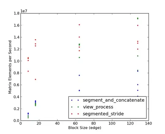
Note that the segmented stride method wins by 3-4x for small block sizes. Only at large block sizes (128 x 128) and very large matrices (2048 x 2048 and larger) does the view processing approach win, and then only by a small percentage. Based on the bake-off, it looks like @eat gets the check-mark! Thanks to both of you for good examples!

Answer 4

Bit late to the game, but this would do overlapping blocks. I haven't done it here, but you could easily adapt for step sizes for shifting the window, I think:

from numpy.lib.stride_tricks import as_strided
def rolling_block(A, block=(3, 3)):
    shape = (A.shape[0] - block[0] + 1, A.shape[1] - block[1] + 1) + block
    strides = (A.strides[0], A.strides[1]) + A.strides
    return as_strided(A, shape=shape, strides=strides)

Answer 5

Even later in the game. There is a Swiss Image processing package called Bob available at: https://www.idiap.ch/software/bob/ It has some python commands for blocks, e.g. bob.ip.base.block which appears to do everything the Matlab command 'blockproc' does. I have not tested it.

There are also interesting commands bob.ip.base.DCTFeatures which incorporates the 'block' capabilities to extract or modify DCT coefficients of an image.

Answer 6

I found this tutorial - The final source code provides exactly the desired functionality! It even should work for any dimensionality (I did not test it) http://www.johnvinyard.com/blog/?p=268

Though the "flatten" option at the very end of the source code seems to be a little buggy. Nevertheless, very nice piece of software!