Plotting a number line in Mathematica

Question

I would like to plot a simple interval on the number line in Mathematica. How do I do this?

Answer 1

For plotting open or closed intervals you could do something like:

intPlot[ss_, {s_, e_}, ee_] := Graphics[{Red, Thickness[.01],
   Text[Style[ss, Large, Red, Bold], {s, 0}],
   Text[Style[ee, Large, Red, Bold], {e, 0}],
   Line[{{s, 0}, {e, 0}}]},
  Axes -> {True, False},
  AxesStyle -> Directive[Thin, Blue, 12],
  PlotRange -> {{ s - .2 Abs@(s - e), e + .2 Abs@(s - e)}, {0, 0}},
  AspectRatio -> .1]

intPlot["[", {3, 4}, ")"]

Edit

Following is the nice extension done by @Simon, probably spoiled by me again trying to solve the overlapping intervals issue.

intPlot[ss_, {s_, e_}, ee_] := intPlot[{{ss, {s, e}, ee}}]
intPlot[ints : {{_String, {_?NumericQ, _?NumericQ}, _String} ..}] :=
 Module[{i = -1, c = ColorData[3, "ColorList"]},
  With[
   {min = Min[ints[[All, 2, 1]]], max = Max[ints[[All, 2, 2]]]},
   Graphics[Table[
     With[{ss = int[[1]], s = int[[2, 1]], e = int[[2, 2]], ee = int[[3]]}, 
       {c[[++i + 1]], Thickness[.01],
       Text[Style[ss, Large, c[[i + 1]], Bold], {s, i}], 
       Text[Style[ee, Large, c[[i + 1]], Bold], {e, i}],
       Line[{{s, i}, {e, i}}]}], {int, ints}], 
    Axes -> {True, False}, 
    AxesStyle -> Directive[Thin, Blue, 12], 
    PlotRange -> {{min - .2 Abs@(min - max), max + .2 Abs@(min - max)}, {0, ++i}}, 
    AspectRatio -> .2]]]

(*Examples*)

intPlot["[", {3, 4}, ")"]
intPlot[{{"(", {1, 2}, ")"}, {"[", {1.5, 4}, ")"}, 
        {"[", {2.5, 7}, ")"}, {"[", {1.5, 4}, ")"}}]

Answer 2

Here's an ugly solution using RegionPlot. Open limits are represented using dotted lines and closed limits with full lines

numRegion[expr_, var_Symbol:x, range:{xmin_, xmax_}:{0, 0}, opts:OptionsPattern[]] :=
            Module[{le=LogicalExpand[Reduce[expr,var,Reals]],
                    y, opendots, closeddots, max, min, len},
 opendots =   Cases[Flatten[le/.And|Or->List], n_<var|n_>var|var<n_|var>n_:>n];
 closeddots = Cases[Flatten[le/.And|Or->List], n_<=var|n_>=var|var<=n_|var>=n_:>n];
 {max, min} = If[TrueQ[xmin < xmax], {xmin, xmax}, 
                 {Max, Min}@Cases[le, _?NumericQ, Infinity] // Through];
 len = max - min;
 RegionPlot[le && -1 < y < 1, {var, min-len/10, max+len/10}, {y, -1, 1},
            Epilog -> {Thick, Red, Line[{{#,1},{#,-1}}]&/@closeddots,
                       Dotted, Line[{{#,1},{#,-1}}]&/@opendots},
            Axes -> {True,False}, Frame->False, AspectRatio->.05, opts]]

An example reducing an absolute value:

numRegion[Abs[x] < 2]

Can use any variable:

numRegion[0 < y <= 1 || y >= 2, y]

Reduces extraneous inequalities, compare the following:

GraphicsColumn[{numRegion[0 < x <= 1 || x >= 2 || x < 0],
                numRegion[0 < x <= 1 || x >= 2 || x <= 0, x, {0, 2}]}]

Answer 3

Here's another attempt that draws number lines with the more conventional white and black circles, although any graphics element that you want can be easily swapped out.

It relies on LogicalExpand[Simplify@Reduce[expr, x]] and Sort to get the expression into something resembling a canonical form that the replacement rules can work on. This is not extensively tested and probably a little fragile. For example if the given expr reduces to True or False, my code does not die gracefully.

numLine[expr_, x_Symbol:x, range:{_, _}:{Null, Null}, 
  Optional[hs:_?NumericQ, 1/30], opts:OptionsPattern[]] := 
 Module[{le = {LogicalExpand[Simplify@Reduce[expr, x]]} /. Or -> List,
   max, min, len, ints = {}, h, disk, hArrow, lt = Less|LessEqual, gt = Greater|GreaterEqual},
  If[TrueQ@MatchQ[range, {a_, b_} /; a < b],
   {min, max} = range,
   {min, max} = Through[{Min, Max}@Cases[le, _?NumericQ, \[Infinity]]]];
  len =Max[{max - min, 1}]; h = len hs;
  hArrow[{x1_, x2_}, head1_, head2_] := {{Thick, Line[{{x1, h}, {x2, h}}]},
                                         Tooltip[head1, x1], Tooltip[head2, x2]};
  disk[a_, ltgt_] := {EdgeForm[{Thick, Black}], 
    Switch[ltgt, Less | Greater, White, LessEqual | GreaterEqual, Black], 
    Disk[{a, h}, h]};
  With[{p = Position[le, And[_, _]]}, 
       ints = Extract[le, p] /. And -> (SortBy[And[##], First] &); 
       le = Delete[le, p]];   
  ints = ints /. (l1 : lt)[a_, x] && (l2 : lt)[x, b_] :> 
     hArrow[{a, b}, disk[a, l1], disk[b, l2]];
  le = le /. {(*_Unequal|True|False:>Null,*)
     (l : lt)[x, a_] :> (min = min - .3 len; 
       hArrow[{a, min}, disk[a, l], 
        Polygon[{{min, 0}, {min, 2 h}, {min - Sqrt[3] h, h}}]]),
     (g : gt)[x, a_] :> (max = max + .3 len; 
       hArrow[{a, max}, disk[a, g], 
        Polygon[{{max, 0}, {max, 2 h}, {max + Sqrt[3] h, h}}]])};
  Graphics[{ints, le}, opts, Axes -> {True, False}, 
   PlotRange -> {{min - .1 len, max + .1 len}, {-h, 3 h}},
   GridLines -> Dynamic[{{#, Gray}} & /@ MousePosition[
                           {"Graphics", Graphics}, None]], 
   Method -> {"GridLinesInFront" -> True}]
  ]

(Note: I had originally tried to use Arrow and Arrowheads to draw the lines - but since Arrowheads automatically rescales the arrow heads with respect to the width of the encompassing graphics, it gave me too many headaches.)

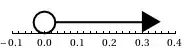
OK, some examples:

numLine[0 < x], 
numLine[0 > x]
numLine[0 < x <= 1, ImageSize -> Medium]

numLine[0 < x <= 1 || x > 2, Ticks -> {{0, 1, 2}}]

numLine[x <= 1 && x != 0, Ticks -> {{0, 1}}]

GraphicsColumn[{
  numLine[0 < x <= 1 || x >= 2 || x < 0],
  numLine[0 < x <= 1 || x >= 2 || x <= 0, x, {0, 2}]
  }]

Edit: Let's compare the above to the output of Wolfram|Alpha

WolframAlpha["0 < x <= 1 or x >= 2 or x < 0", {{"NumberLine", 1}, "Content"}]
WolframAlpha["0 < x <= 1 or x >= 2 or x <= 0", {{"NumberLine", 1}, "Content"}]

Note (when viewing the above in a Mathematica session or the W|A website) the fancy tooltips on the important points and the gray, dynamic grid lines. I've stolen these ideas and incorporated them into the edited numLine[] code above.

The output from WolframAlpha is not quite a normal Graphics object, so it's hard to modify its Options or combine using Show. To see the various numberline objects that Wolfram|Alpha can return, run WolframAlpha["x>0", {{"NumberLine"}}] - "Content", "Cell" and "Input" all return basically the same object. Anyway, to get a graphics object from

wa = WolframAlpha["x>0", {{"NumberLine", 1}, "Content"}]

you can, for example, run

Graphics@@First@Cases[wa, GraphicsBox[__], Infinity, 1]

Then we can modify the graphics objects and combine them in a grid to get

Answer 4

Starting with Mathematica 10, there is NumberLinePlot available.

Answer 5

The previous ugly solution has helped me to develop the InequalityPlot function to solve and plotting inequalities in two variables.

InequalityPlot[ineq_, {x_Symbol, xmin_, xmax_},{y_Symbol, ymin_, ymax_},
  opts : OptionsPattern[Join[Options[ContourPlot],
    Options[RegionPlot], {CurvesColor -> RGBColor[1, .4, .2]}]]] :=
 Module[{le = LogicalExpand[ineq], opencurves, closedcurves, curves},
  opencurves = Cases[Flatten[{le /. And | Or -> List}],
   lexp_ < rexp_ | lexp_ > rexp_ | lexp_ < rexp_ | lexpr_ > rexp_ :>
    {lexp == rexp, Dashing[Medium]}];
  closedcurves = Cases[Flatten[{le /. And | Or -> List}],
   lexp_ <= rexp_ | lexp_ >= rexp_ | lexp_ <= rexp_ | lexp_ >= rexp_ :>
    {lexp == rexp, Dashing[None]}];
  curves = Join[opencurves, closedcurves];
  Show[  RegionPlot[ineq, {x, xmin, xmax}, {y, ymin, ymax},
    BoundaryStyle -> None,
    Evaluate[Sequence @@ FilterRules[{opts}, Options[RegionPlot]]]],
   ContourPlot[First[#] // Evaluate, {x, xmin, xmax}, {y, ymin, ymax},
      ContourStyle -> Directive[OptionValue[CurvesColor], Last[#]],
      Evaluate[Sequence @@ FilterRules[{opts},
         Options[ContourPlot]]]] & /@ curves  ]
 ]

Here are two examples:

InequalityPlot[0.5 <= x^2 + y^2 < 1, {x, -1, 1}, {y, -1, 1}]

InequalityPlot[x^2 + y^2 < 0.5 && x + y <= 0.5,{x, -1, 1}, {y, -1, 1}]

Answer 6

Do a regular Plot, and set Axes -> {True, False} (and hide the bounding box if one exists, which one usually does not). Adjust image size or aspect ratio as appropriate.

e.g.

Plot[
    Piecewise[{
        {0, And[0<x, x<1]}
    }],
    {x,-1,2},
    Axes -> {True, False}        
]

You can use Show to combine this with an imagine of open-and-closed dots.

There is a small chance you may have to pass in Indeterminate or some other special value as the second argument to Piecewise (or else it defaults to 0), if you do not properly set your line width or similar plotting styles; or, alternatively but more assuredly, set the value to 999 and PlotRange -> {{-1,2},{-.1,.1}}.