How to visualize a keras neural network with trained weights?

Question

I have created a sequential model using keras package similar to this:

from keras.layers import Dense
from keras.models import Sequential

model = Sequential()

# Adding the input layer and the first hidden layer
model.add(Dense(6, activation='relu',input_dim = 11))

# Adding the second hidden layer (The real model contains many hidden layers)
model.add(Dense(6,activation='relu')) 
# Adding the output layer
model.add(Dense( 1, activation = 'sigmoid'))

Then I used keras visualizer to get a visualization of the neural network without weights.

# Compiling the ANN
classifier.compile(optimizer = 'Adamax', loss = 'binary_crossentropy',metrics=['accuracy'])
model_history=classifier.fit(X_train, y_train.to_numpy(), batch_size = 10, epochs = 100)

I want to print trained weights of the model for this kind of visualization. Is there any library or module that I can use for that? Any suggestion will be helpful. Here is the picture of the designed neural network without printing weights.

Answer 1

I want to print trained weights of the model to this kind of visualization. Is there any library or module that I can use for that?

Option1: deepreplay

There is a workaround in the form of package\module so-called Deep Replay you can import as a library for resolving your problem.

Thanks to this package, you can visualize\animate and the most probably print trained weights using the following example:

# install FFMPEG (to generate animations)
#!apt-get install ffmpeg

# install actual deepreplay package
#!pip install deepreplay

from keras.initializers import glorot_normal, glorot_uniform, he_normal, he_uniform
from keras.layers import Dense
from keras.models import Sequential
from deepreplay.callbacks import ReplayData
from deepreplay.datasets.ball import load_data
from deepreplay.plot import compose_plots, compose_animations
from deepreplay.replay import Replay

from matplotlib import pyplot as plt

plt.rcParams['animation.ffmpeg_path'] = '/usr/bin/ffmpeg'

X, y = load_data(n_dims=10)

activation = 'relu'
initializer_name = 'he_uniform'
initializer = eval(initializer_name)(seed=13)
title = 'Activation: ReLU - Initializer: {}'.format(initializer_name)
group_name = 'relu_{}'.format(initializer_name)
filename = f'{group_name}_{initializer_name}_{activation}_weight_initializers.h5'

# Model builder function
def build_model(n_layers, input_dim, units, activation, initializer):
    if isinstance(units, list):
        assert len(units) == n_layers
    else:
        units = [units] * n_layers

    model = Sequential()
    # Adds first hidden layer with input_dim parameter
    model.add(Dense(units=units[0],
                    input_dim=input_dim,
                    activation=activation,
                    kernel_initializer=initializer,
                    name='h1'))

    # Adds remaining hidden layers
    for i in range(2, n_layers + 1):
        model.add(Dense(units=units[i-1],
                        activation=activation,
                        kernel_initializer=initializer,
                        name='h{}'.format(i)))

    # Adds output layer
    model.add(Dense(units=1, activation='sigmoid', kernel_initializer=initializer, name='o'))
    # Compiles the model
    model.compile(loss='binary_crossentropy', optimizer='sgd', metrics=['acc'])
    return model


replaydata = ReplayData(X, y, filename=filename, group_name=group_name)

# Create the MLP model with 5 layers within 10 input neurons and 100 unists in hidden and output layers
model = build_model(n_layers=5, input_dim=10, units=100, activation=activation, initializer=initializer)

# fit the model over 10 epochs with batch size of 16
model.fit(X, y, epochs=10, batch_size=16, callbacks=[replaydata])

# Plot the results
replay = Replay(replay_filename=filename, group_name=group_name)

fig = plt.figure(figsize=(12, 6))
ax_zvalues = plt.subplot2grid((2, 2), (0, 0))
ax_weights = plt.subplot2grid((2, 2), (0, 1))
ax_activations = plt.subplot2grid((2, 2), (1, 0))
ax_gradients = plt.subplot2grid((2, 2), (1, 1))

wv = replay.build_weights(ax_weights)
gv = replay.build_gradients(ax_gradients)

# Z-values
zv = replay.build_outputs(ax_zvalues, before_activation=True,
                          exclude_outputs=True, include_inputs=False)
# Activations
av = replay.build_outputs(ax_activations, exclude_outputs=True, include_inputs=False)

# Save plots
fig = compose_plots([zv, wv, av, gv], epoch=0, title=title)
fig.savefig('part2.png', format='png', dpi=120)

# Animate & save mp4
sample_anim = compose_animations([zv, wv, av, gv])
sample_anim.save('part2.mp4', dpi=120, fps=5)

visulize output results using violin plots over 10 epochs for simple: 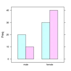So the top right subplot shows Weights change through the layers over ten epochs. The other subplots illustrate the performance of Z-values, Activation functions, and Gradients changes.

Note1: if you are interested to interpret violin plots, please check these posts: post1 , post2, post3

Note2: Please notice that the training process starts with some initializers, which can have different weighing at the beginning. The common initialization schemes are as follows:

• Random
• Xavier / Glorot
• He

By default, kernel initializer is glorot_uniform when you use keras module (reference), but you can check this post and this paper Understanding the difficulty of training deep feedforward neural networks for further info. It is also possible to initialize weights in NN manually. You can check this post.

Note3: Recently, this package has a bug and can't be implemented in Google Colab Notebook, which is still an open issue; its GH Repo as well as post in SoF. So it is better to try it on your own local machine, hopefully.

Option2:wandb

There is another ML-based tool, so-called W&B (Weights and Biases) you can import as a library for resolving your problem.

once you sign-up and login into your account based on instructions, you can use this API to track and visualize all the pieces of your ML pipeline, including Weights and Biases and other parameters in your pipeline:

import wandb
from wandb.keras import WandbCallback

# Step1: Initialize W&B run
wandb.init(project='project_name')

# 2. Save model inputs and hyperparameters
config = wandb.config
config.learning_rate = 0.01

# Model training code here ...
import tensorflow as tf
from tensorflow import keras
loss=tf.keras.losses.MeanSquaredError()
Optimiser=tf.keras.optimizers.Adam(learning_rate =0.001)
model.compile(loss=loss, optimizer=Optimiser, metrics=['accuracy'])
wandb.log({"loss": loss})

# Step 3: Add WandbCallback 
model.fit(X, y, epochs=10, batch_size=16, callbacks=[WandbCallback()])

once you run your model, you can check graph info in the Model section which is selected\shown on the left side with blue color:

hope this answer helps you out, and if it is so, you can accept it as an answer ✅.