On cell D2 put the following formula:
=LET(set, A2:B5, m, COLUMNS(set), seq, SEQUENCE(m,1),
 CUMULATE, LAMBDA(x, SCAN(0, x, LAMBDA(acc,item, acc+item))),
 DROP(REDUCE(0,seq, LAMBDA(acc,idx, HSTACK(acc, CUMULATE(INDEX(set,,idx))))),,1)
)
Here is the output:

It also works without removing the first column via DROP if the accumulator is initialized properly, with the cumulative sum of the first column, as follow:
=LET(set, A2:B5, m, COLUMNS(set), seq, SEQUENCE(m,1),
 CUMULATE, LAMBDA(x, SCAN(0, x, LAMBDA(acc,item, acc+item))),
 REDUCE(0,seq, LAMBDA(acc,idx, IF(idx = 1, CUMULATE(INDEX(set,,idx)),
  HSTACK(acc, CUMULATE(INDEX(set,,idx))))))
)
Update
An alternative is also the following solution using MAP with the same shape as the input range, so there is no need to add columns via DROP/REDUCE/HSTACK pattern:
=LET(n, ROWS(A2:B5), m, COLUMNS(A2:B5),
  rows, MAKEARRAY(n, m, LAMBDA(r, c, r)),cols, MAKEARRAY(n, m, LAMBDA(r, c, c)),
  MAP(rows, cols, LAMBDA(r, c, SUM(INDEX(A2:B5, 1, c):INDEX(A2:B5, r, c)) ))
)
Note: You cannot pass a name from LET to represent the range A2:B5 inside a LAMBDA function for using a function/operation that expects a range such as building a range as follow: INDEX() : INDEX(). Check the answer from @JosWoolley to this question: Using name variable from LET produces #VALUE! inside MAP using SUM with the range defined as INDEX : INDEX
Explanation
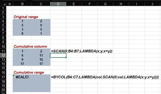
BYCOL returns one cell per column, that is why you get #CALC! error related to Nested Array Error. It can be circumvent using DROP/REDUCE/HSTACK pattern, explained here for example: how to transform a table in Excel from vertical to horizontal but with different length answer provided by @DavidLeal.
For your particular case, we need to calculate the cumulative sum for each column. We created a user LAMBDA function for that: CUMULATE:
LAMBDA(x, SCAN(0, x, LAMBDA(acc, item, acc+item)))
Now we use the pattern to iterate over all columns. REDUCE function needs an input array, so we create a seq name with the column positions. We can access to each column of the input range (set), via INDEX(set,,idx), where idx represents the column number.
Now we use the pattern DROP/REDUCE/HSTACK explained in the above link to generate each column:
DROP(REDUCE(0, arr, LAMBDA(acc, x, HSTACK(acc, func(x)))),,1)
In our case func(x) will be the user LAMBDA function we just created: CUMULATE, so in our case it will be:
DROP(REDUCE(0,seq, LAMBDA(acc,idx, HSTACK(acc, CUMULATE(INDEX(set,,idx))))),,1)
What it does is to invoke for each column of set the CUMULATE LAMBDA function and via HSTACK appends the column created on each iteration. The variable acc represents the accumulator, so we start with initial value of the accumulator 0, then we add recursively via HSTACK the following columns. Finally we need to remove the first column via DROP(result,,1) that represents the first iteration that doesn't calculate the cumulative sum and just generate a column like this one:
0
#N/A
#N/A
#N/A
Note: If an array has fewer rows than the maximum width of the selected arrays, HSTACK returns a #N/A error in the additional rows. That is why you get such values. Bottom line, the first column needs to be removed, because we didn't initialized with a valid value the first iteration. I provided a second alternative that doesn't require to remove this column but at the end is a more verbose formula. It is a matter of personal preferences.


