Optimizing size of eps/pdf files generated by Mathematica

Question

How to optimize size of an eps or pdf file generated by Mathematica?

It is common that the file size is 50-100x bigger that it should be (an example below). For some applications (e.g. putting a figure in a publication, or even more - putting it on a large poster) I need to have axes in vector graphics, so using raster graphics for everything is not the best option for me.

Every practical solution (either with setting the right options in Mathematica or with doing further conversions in other applications) will be appreciated.

For example the following code producing an eps figure of:

plot = ListDensityPlot[
Table[Random[], {100}, {100}],
InterpolationOrder -> 0]

Export["testplot.eps", plot]
Export["testplot.pdf", plot]

produces an eps file of size of 3.3MB and a pdf size of 5MB (on Mathematica 7 on Mac OS X 10.6, if it makes a difference).

For a comparison, a 3x3 plot with the same axes has 8kB (pdf) to 20kB (eps). 100x100 points is 30kB in bmp (and a bit less in png).

The issue is the same for other types of plots, with the emphasis on ListPlot3D.

Strongly related thread (but about 3D graphics): "[Mathematica: Rasters in 3D graphics](http://stackoverflow.com/q/6301676/590388)." — Alexey Popkov, Oct 31 '11 at 17:45

score 5 · Accepted Answer · edited Jun 20 '20 at 09:12

You may have figured out how to apply Alexey's answer in the link he provided. But in case you are having trouble here I provide how I apply the technique to 2D graphics.

I have found the hard way that if you want to create a good plot you need to be very specific to Mathematica. For this reason, as you may have noticed in my post Rasters in 3D I created an object specifying all the options so that Mathematica can be happy.

in = 72;
G2D = Graphics[{},
   AlignmentPoint -> Center, 
   AspectRatio -> 1,
   Axes -> False,
   AxesLabel -> None,
   BaseStyle -> {FontFamily -> "Arial", FontSize -> 12},
   Frame -> True,
   FrameStyle -> Directive[Black],
   FrameTicksStyle -> Directive[10, Black],
   ImagePadding -> {{20, 5}, {15, 5}},
   ImageSize -> 5 in, 
   LabelStyle -> Directive[Black],
   PlotRange -> All,
   PlotRangeClipping -> False,
   PlotRangePadding -> Scaled[0.02]
];

I should mention here that you must specify ImagePadding. If you set it to all your eps file will be different from what Mathematica shows you. In any case, I think having this object allows you to change properties much easily.

Now we can move on to your problem:

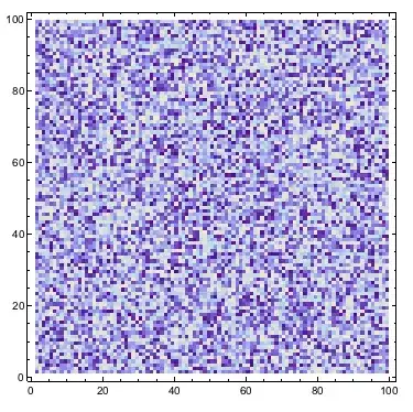
plot = ListDensityPlot[
  Table[Random[], {100}, {100}],
  InterpolationOrder -> 0,
  Options[G2D]
]

Output

The following separates the axes and the raster and combines them into result:

axes = Graphics[{}, AbsoluteOptions[plot]];
fig = Show[plot, FrameStyle -> Directive[Opacity[0]]];
fig = Magnify[fig, 5];
fig = Rasterize[fig, Background -> None];
axes = First@ImportString[ExportString[axes, "PDF"], "PDF"];
result = Show[axes, Epilog -> Inset[fig, {0, 0}, {0, 0}, ImageDimensions[axes]]]

Output2

The only difference here, which at this point I cannot explain is the axes labels, they have the decimal point. Finally, we export them:

Export["Result.pdf", result];
Export["Result.eps", result];

The result are files of sizes 115 Kb for the pdf file and 168 Kb for the eps file.

UPDATE:

If you are using Mathematica 7 the eps file will not come up correctly. All you will see is your main figure with black on the sides. This is a bug in version 7. This however is fixed in Mathematica 8.

I had mentioned previously that I did not know why the axes label were different. Alexey Popkov came up with a fix for that. To create axes, fig and result use the following:

axes = Graphics[{}, FilterRules[AbsoluteOptions[plot], Except[FrameTicks]]];
fig = Show[plot, FrameStyle -> Directive[Opacity[0]]];
fig = Magnify[fig, 5];
fig = Rasterize[fig, Background -> None];
axes = First@ImportString[ExportString[axes, "PDF"], "PDF"];
result = Show[axes, Epilog -> Inset[fig, {0, 0}, {0, 0}, ImageDimensions[axes]]]

It works, thank you a lot! On my computer the sizes are: 180kB (eps) and 123kb (pdf). — Piotr Migdal, Nov 01 '11 at 20:30
However, for eps file the background is black, covering the axes; `Export["Result.eps", result, Background -> White]` does not help. For pdf file everything works fine. — Piotr Migdal, Nov 01 '11 at 20:44
@PiotrMigdal, I think this might be because you are using MMA7. This is something I pointed out in Rasters in 3D. If you switch to MMA8, then the eps file should come out ok. This is just a bug in version 7 I believe. Glad this is of help. — jmlopez, Nov 01 '11 at 21:13
The axes labels have decimal point because of a bug in `AbsolutOptions` - just look at `FrameTicks /. AbsoluteOptions[plot]`. — Alexey Popkov, Nov 04 '11 at 03:14
@AlexeyPopkov, Any idea how to fix this? In the past I've been lucky that the labels come out correctly since they are decimals most of the time. For the few that come out incorrectly I usually fix the `FrameTicks` one by one since there are not many. — jmlopez, Nov 04 '11 at 17:04
Use `FilterRules[AbsoluteOptions[plot], Except[FrameTicks]]` instead of `AbsoluteOptions[plot]` as a workaround. — Alexey Popkov, Nov 04 '11 at 17:57
For me, it was not working until I set PlotRange manually and what was the most important, I had to specify also 3rd dimension PlotRange, although I was plotting 2D plot. But I got amazing result. ListPlot with more than 80 000 values which had 5,3MB has after application of this hint 83kB. Thanks! — matejuh, Apr 22 '12 at 09:23
@matejuh, I can't say for sure that everything is going to work. Usually you have to be very specific about everything with Mathematica. Glad you got it work with good results. — jmlopez, Apr 25 '12 at 21:32

score 3 · Answer 2 · answered Oct 31 '11 at 14:33

3

I have had some success with both of the following:

(1) Rasterizing plots before saving. Quality is generally reasonable, size drops considerably.

(2) I Save to postscript, then (I'm on a Linux machine) use ps2pdf to get the pdf. This tends to be significantly smaller than saving directly to pdf from Mathematica.

Daniel Lichtblau

answered Oct 31 '11 at 14:33

Daniel Lichtblau

6,854
1
23
30

Thanks. Unfortunately, as I tested it `ps2pdf plot.eps` yields in a 7.7MB file, so it makes things even worse. – Piotr Migdal Oct 31 '11 at 15:19
@Piotr Migdal Ouch. I've never had that happen. Mine always seem to get smaller by a factor of 10 or so. – Daniel Lichtblau Oct 31 '11 at 15:38

DavidC · Answer 3 · 2011-10-31T14:19:09.787

2

ImageResolution works well for .pdf but I haven't had success with .eps.

Export["testplot600.pdf", plot, ImageResolution -> 600]

The output size is 242 KB for 600 dpi and 94 KB for 300 dpi. You can also set ImageSize for Export.

If you want to go the third-party route, I'd recommend GraphicConverter. It is very reliable and has many many options.

edited Oct 31 '11 at 14:19

answered Oct 31 '11 at 13:48

DavidC

3,056
1
20
30

1

Thanks. But actually, I already know this option and it is not a thing I am looking for. `ImageResolution -> res` is a rasterization of the data points and the axes alike. – Piotr Migdal Oct 31 '11 at 14:25

Optimizing size of eps/pdf files generated by Mathematica

3 Answers3

UPDATE: