How to add a single colobar that will show the data from 2 different subplot

Question

What i wanna do is adding a single colorbar (at the right side of the figure shown below), that will show the colorbar for both subplots (they are at the same scale).

Another thing doesn't really make sense for me is why the lines I try to draw on the end of the code are not drawn (they are supposed to be horizontal lines on the center of both plots)

Thanks for the help.

Here are the code:

 idx=0
b=plt.psd(dOD[:,idx],Fs=self.fs,NFFT=512)
B=np.zeros((2*len(self.Chan),len(b[0])))
B[idx,:]=20*log10(b[0])

c=plt.psd(dOD_filt[:,idx],Fs=self.fs,NFFT=512)
C=np.zeros((2*len(self.Chan),len(b[0])))
C[idx,:]=20*log10(c[0])

for idx in range(2*len(self.Chan)):
    b=plt.psd(dOD[:,idx],Fs=self.fs,NFFT=512)
    B[idx,:]=20*log10(b[0])

    c=plt.psd(dOD_filt[:,idx],Fs=self.fs,NFFT=512)
    C[idx,:]=20*log10(c[0])

## Calculate the color scaling for the imshow()    
aux1 = max(max(B[i,:]) for i in range(size(B,0)))
aux2 = min(min(B[i,:]) for i in range(size(B,0)))
bux1 = max(max(C[i,:]) for i in range(size(C,0)))
bux2 = min(min(C[i,:]) for i in range(size(C,0)))
scale1 = 0.75*max(aux1,bux1)
scale2 = 0.75*min(aux2,bux2)


fig, axes = plt.subplots(nrows=2, ncols=1,figsize=(7,7))#,sharey='True')
fig.subplots_adjust(wspace=0.24, hspace=0.35)

ii=find(c[1]>=frange)[0]
## Making the plots
cax=axes[0].imshow(B, origin = 'lower',vmin=scale2,vmax=scale1)
axes[0].set_ylim((0,2*len(self.Chan)))
axes[0].set_xlabel(' Frequency (Hz) ')
axes[0].set_ylabel(' Channel Number ') 
axes[0].set_title('Pre-Filtered')
cax2=axes[1].imshow(C, origin = 'lower',vmin=scale2,vmax=scale1)
axes[1].set_ylim(0,2*len(self.Chan))
axes[1].set_xlabel(' Frequency (Hz) ')
axes[1].set_ylabel(' Channel Number ')
axes[1].set_title('Post-Filtered')

axes[0].annotate('690nm', xy=((ii+1)/2, len(self.Chan)/2-1), 
        xycoords='data', va='center', ha='right')
axes[0].annotate('830nm', xy=((ii+1)/2, len(self.Chan)*3/2-1 ), 
        xycoords='data', va='center', ha='right')
axes[1].annotate('690nm', xy=((ii+1)/2, len(self.Chan)/2-1), 
        xycoords='data', va='center', ha='right')
axes[1].annotate('830nm', xy=((ii+1)/2, len(self.Chan)*3/2-1 ), 
        xycoords='data', va='center', ha='right')


axes[0].axis('tight')
axes[1].axis('tight')


## Set up the xlim to aprox frange Hz
axes[0].set_xlim(left=0,right=ii)
axes[1].set_xlim(left=0,right=ii)

## Make the xlabels become the actual frequency number
ticks = linspace(0,ii,10)
tickslabel = linspace(0.,frange,10)
for i in range(10):
    tickslabel[i]="%.1f" % tickslabel[i]
axes[0].set_xticks(ticks)
axes[0].set_xticklabels(tickslabel)
axes[1].set_xticks(ticks)
axes[1].set_xticklabels(tickslabel)

## Draw a line to separate the two different wave lengths, and name each region
l1 = Line2D([0,frange],[28,28],ls='-',color='black')
axes[0].add_line(l1)
axes[1].add_line(l1)

And here the figure it makes: enter image description here

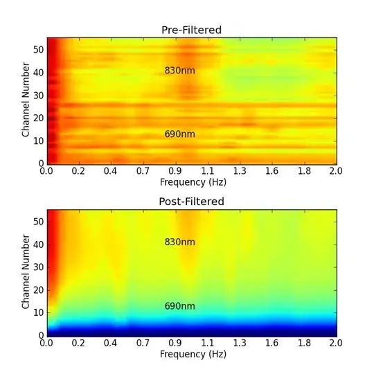
If any more info are needed, just ask.

oz123 · Accepted Answer · 2012-03-28T20:18:19.060

Basically, figure.colorbar() is good for both images, as long as their are not with too different scales. So you could let matplotlib do it for you... or you manually position your colorbar on axes inside the images. Here is how to control the location of the colorbar:

import numpy as np
from matplotlib import pyplot as plt

A = np.random.random_integers(0, 10, 100).reshape(10, 10)
B = np.random.random_integers(0, 10, 100).reshape(10, 10)

fig = plt.figure()
ax1 = fig.add_subplot(221)
ax2 = fig.add_subplot(222)

mapable = ax1.imshow(A, interpolation="nearest")
cax = ax2.imshow(A, interpolation="nearest")

# set the tickmarks *if* you want cutom (ie, arbitrary) tick labels:
cbar = fig.colorbar(cax, ax=None)

fig = plt.figure(2)
ax1 = fig.add_subplot(121)
ax2 = fig.add_subplot(122)
mapable = ax1.imshow(A, interpolation="nearest")
cax = ax2.imshow(A, interpolation="nearest")
# on the figure total in precent l    b      w , height 
ax3 = fig.add_axes([0.1, 0.1, 0.8, 0.05]) # setup colorbar axes. 
# put the colorbar on new axes
cbar = fig.colorbar(mapable,cax=ax3,orientation='horizontal')

plt.show()

Note ofcourse you can position ax3 as you wish, on the side, on the top, where ever, as long as it is in the boundaries of the figure.

I don't know why your line2D is not appearing.

I added to my code before plt.show() the following and everything is showing:

from mpl_toolkits.axes_grid1 import anchored_artists
from matplotlib.patheffects import withStroke
txt = anchored_artists.AnchoredText("SC",
                                    loc=2,
                                    frameon=False,
                                    prop=dict(size=12))
if withStroke:
    txt.txt._text.set_path_effects([withStroke(foreground="w",
                                               linewidth=3)])
ax1.add_artist(txt)


## Draw a line to separate the two different wave lengths, and name each region
l1 = plt.Line2D([-1,10],[5,5],ls='-',color='black',lineswidth=10)
ax1.add_line(l1)

Color bar on axes WithLine

The colorbar method realyl worked out.. Just had to use a subplot_adjust since i was using axis('tight') and i wanted the colobar to be on the right side..... About the Line2D, i tried basically everything and it just won't show ;/... Any other methods on showing lines?? Anyways, thanks alot.. — Rodrigo Forti, Mar 28 '12 at 21:40
Figured out a way of showing up the lines.. It had something to do with how i called the axes.... All i had to do is change the lines where i add the axes to :{ for (i), ax in np.ndenumerate(axes): l1 = plt.Line2D([0,ii],[28,28],ls='-',color='black') ax.add_line(l1)} — Rodrigo Forti, Mar 28 '12 at 23:20

How to add a single colobar that will show the data from 2 different subplot

1 Answers1

Linked