Plot probability heatmap/hexbin with different sized bins

Question

This is related to another question: Plot weighted frequency matrix.

I have this graphic (produced by the code below in R):

#Set the number of bets and number of trials and % lines
numbet <- 36 
numtri <- 1000 
#Fill a matrix where the rows are the cumulative bets and the columns are the trials
xcum <- matrix(NA, nrow=numbet, ncol=numtri)
for (i in 1:numtri) {
x <- sample(c(0,1), numbet, prob=c(5/6,1/6), replace = TRUE)
xcum[,i] <- cumsum(x)/(1:numbet)
}
#Plot the trials as transparent lines so you can see the build up
matplot(xcum, type="l", xlab="Number of Trials", ylab="Relative Frequency", main="", col=rgb(0.01, 0.01, 0.01, 0.02), las=1)

I very much like the way that this plot is built up and shows the more frequent paths as darker than the rarer paths (but it is not clear enough for a print presentation). What I would like to do is to produce some kind of hexbin or heatmap for the numbers. On thinking about it, it seems that the plot will have to incorporate different sized bins (see my back of the envelope sketch):

My question then: If I simulate a million runs using the code above, how can I present it as a heatmap or hexbin, with the different sized bins as shown in the sketch?

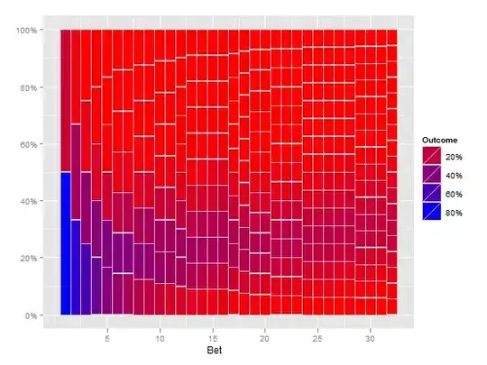
To clarify: I do not want to rely on transparency to show the rarity of a trial passing through a part of the plot. Instead I would like to denote rarity with heat and show a common pathway as hot (red) and a rare pathway as cold (blue). Also, I do not think the bins should be the same size because the first trial has only two places where the path can be, but the last has many more. Hence the fact I chose a changing bin scale, based on that fact. Essentially I am counting the number of times a path passes through the cell (2 in col 1, 3 in col 2 etc) and then colouring the cell based on how many times it has been passed through.

UPDATE: I already had a plot similar to @Andrie, but I am not sure it is much clearer than the top plot. It is the discontinuous nature of this graph, that I do not like (and why I want some kind of heatmap). I think that because the first column has only two possible values, that there should not be a huge visual gap between them etc etc. Hence why I envisaged the different sized bins. I still feel that the binning version would show large number of samples better.

Update: This website outlines a procedure to plot a heatmap:

To create a density (heatmap) plot version of this we have to effectively enumerate the occurrence of these points at each discrete location in the image. This is done by setting a up a grid and counting the number of times a point coordinate "falls" into each of the individual pixel "bins" at every location in that grid.

Perhaps some of the information on that website can be combined with what we have already?

Update: I took some of what Andrie wrote with some of this question, to arrive at this, which is quite close to what I was conceiving:

numbet <- 20
numtri <- 100
prob=1/6
#Fill a matrix 
xcum <- matrix(NA, nrow=numtri, ncol=numbet+1)
for (i in 1:numtri) {
  x <- sample(c(0,1), numbet, prob=c(prob, 1-prob), replace = TRUE)
  xcum[i, ] <- c(i, cumsum(x)/cumsum(1:numbet))
}
colnames(xcum) <- c("trial", paste("bet", 1:numbet, sep=""))

mxcum <- reshape(data.frame(xcum), varying=1+1:numbet, 
  idvar="trial", v.names="outcome", direction="long", timevar="bet")

 #from the other question
 require(MASS)
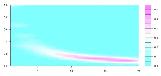
dens <- kde2d(mxcum$bet, mxcum$outcome)
filled.contour(dens)

I don't quite understand what's going on, but this seems to be more like what I wanted to produce (obviously without the different sized bins).

Update: This is similar to the other plots here. It is not quite right:

plot(hexbin(x=mxcum$bet, y=mxcum$outcome))

Last try. As above:

image(mxcum$bet, mxcum$outcome)

This is pretty good. I would just like it to look like my hand-drawn sketch.

Answer 1

Edit

I think the following solution does what you ask for.

(Note that this is slow, especially the reshape step)

numbet <- 32
numtri <- 1e5
prob=5/6
#Fill a matrix 
xcum <- matrix(NA, nrow=numtri, ncol=numbet+1)
for (i in 1:numtri) {
  x <- sample(c(0,1), numbet, prob=c(prob, 1-prob), replace = TRUE)
  xcum[i, ] <- c(i, cumsum(x)/cumsum(1:numbet))
}
colnames(xcum) <- c("trial", paste("bet", 1:numbet, sep=""))

mxcum <- reshape(data.frame(xcum), varying=1+1:numbet, 
  idvar="trial", v.names="outcome", direction="long", timevar="bet")


library(plyr)
mxcum2 <- ddply(mxcum, .(bet, outcome), nrow)
mxcum3 <- ddply(mxcum2, .(bet), summarize, 
                ymin=c(0, head(seq_along(V1)/length(V1), -1)), 
                ymax=seq_along(V1)/length(V1),
                fill=(V1/sum(V1)))
head(mxcum3)

library(ggplot2)

p <- ggplot(mxcum3, aes(xmin=bet-0.5, xmax=bet+0.5, ymin=ymin, ymax=ymax)) + 
    geom_rect(aes(fill=fill), colour="grey80") + 
    scale_fill_gradient("Outcome", formatter="percent", low="red", high="blue") +
    scale_y_continuous(formatter="percent") +
    xlab("Bet")

print(p)

Answer 2

FYI: This is more of an extended comment than an answer.

To me, this new plot looks like a stacked bar where each bar's height is equal to the intersection points of the upper and lower line at the next trial.

The way that I would approach this is to treat "Trials" as a categorical variable. Then we can search each row of xcum for elements that are equal. If they are, then we can consider this to be a point of intersection whose minima also represents the multiple defining the height of our bars.

x <- t(xcum)
x <- x[duplicated(x),]
x[x==0] <- NA

Now we have the multiples of the actual points, we need to figure out how to take it to the next step and find a way of binning the information. That means we need to make a decision about how many points will represent each grouping. Let's write some points out for posterity.

Trial 1 (2) = 1, 0.5 # multiple = 0.5
Trial 2 (3) = 1, 0.66, 0.33 #  multiple = 0.33
Trial 3 (4) = 1, 0.75, 0.5, 0.25 # multiple = 0.25
Trial 4 (5) = 1, 0.8,  0.6, 0.4, 0.2 # multiple = 0.2
Trial 5 (6) = 1, 0.8333335, 0.6666668, 0.5000001, 0.3333334, 0.1666667
... 
Trial 36 (35) = 1, 0.9722223, ..., 0.02777778 # mutiple = 0.05555556 / 2

In other words, for each Trial there are n-1 points to plot. In your drawing you have 7 bins. So we need to figure out the multiples for each bin.

Let's cheat and divide the last two columns by two, we know from visual inspection that the minima is lower than 0.05

x[,35:36] <- x[,35:36] / 2

Then find the minimum of each column:

x <- apply(x, 2, function(x) min(x, na.rm=T))[-1] # Drop the 1
x <- x[c(1,2,3,4,8,17,35)] # I'm just guessing here by the "look" of your drawing. 

The clearest way to do this is to create each bin separately. Obviously, this could be done automatically later. Remembering that each point is

bin1 <- data.frame(bin = rep("bin1",2), Frequency = rep(x[1],2))
bin2 <- data.frame(bin = rep("bin2",3), Frequency = rep(x[2],3))
bin3 <- data.frame(bin = rep("bin3",4), Frequency = rep(x[3],4))
bin4 <- data.frame(bin = rep("bin4",5), Frequency = rep(x[4],5))
bin5 <- data.frame(bin = rep("bin5",9), Frequency = rep(x[5],9))
bin6 <- data.frame(bin = rep("bin6",18), Frequency = rep(x[6],18))
bin7 <- data.frame(bin = rep("bin7",36), Frequency = rep(x[7],36))

df <- rbind(bin1,bin2,bin3,bin4,bin5,bin6,bin7)
ggplot(df, aes(bin, Frequency, color=Frequency)) + geom_bar(stat="identity", position="stack")