Extract contours from ContourPlot in Mathematica

Question

I have a function f(x,y) of two variables, of which I need to know the location of the curves at which it crosses zero. ContourPlot does that very efficiently (that is: it uses clever multi-grid methods, not just a brute force fine-grained scan) but just gives me a plot. I would like to have a set of values {x,y} (with some specified resolution) or perhaps some interpolating function which allows me to get access to the location of these contours.

Have thought of extracting this from the FullForm of ContourPlot but this seems to be a bit of a hack. Any better way to do this?

Szabolcs · Accepted Answer · 2011-07-25T13:13:41.273

If you end up extracting points from ContourPlot, this is one easy way to do it:

points = Cases[
  Normal@ContourPlot[Sin[x] Sin[y] == 1/2, {x, -3, 3}, {y, -3, 3}],
  Line[pts_] -> pts,
  Infinity
]

Join @@ points (* if you don't want disjoint components to be separate *)

EDIT

It appears that ContourPlot does not produce very precise contours. They're of course meant for plotting and are good enough for that, but the points don't lie precisely on the contours:

In[78]:= Take[Join @@ points /. {x_, y_} -> Sin[x] Sin[y] - 1/2, 10]

Out[78]= {0.000163608, 0.0000781187, 0.000522698, 0.000516078, 
0.000282781, 0.000659909, 0.000626086, 0.0000917416, 0.000470424, 
0.0000545409}

We can try to come up with our own method to trace the contour, but it's a lot of trouble to do it in a general way. Here's a concept that works for smoothly varying functions that have smooth contours:

Start from some point (pt0), and find the intersection with the contour along the gradient of f.
Now we have a point on the contour. Move along the tangent of the contour by a fixed step (resolution), then repeat from step 1.

Here's a basic implementation that only works with functions that can be differentiated symbolically:

rot90[{x_, y_}] := {y, -x}

step[f_, pt : {x_, y_}, pt0 : {x0_, y0_}, resolution_] :=
 Module[
  {grad, grad0, t, contourPoint},
  grad = D[f, {pt}];
  grad0 = grad /. Thread[pt -> pt0];
  contourPoint = 
    grad0 t + pt0 /. First@FindRoot[f /. Thread[pt -> grad0 t + pt0], {t, 0}];
  Sow[contourPoint];
  grad = grad /. Thread[pt -> contourPoint];
  contourPoint + rot90[grad] resolution
 ]

result = Reap[
   NestList[step[Sin[x] Sin[y] - 1/2, {x, y}, #, .5] &, {1, 1}, 20]
];

ListPlot[{result[[1]], result[[-1, 1]]}, PlotStyle -> {Red, Black}, 
 Joined -> True, AspectRatio -> Automatic, PlotMarkers -> Automatic]

Illustration of the contour finding method

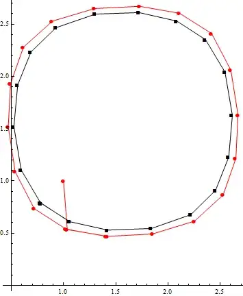
The red points are the "starting points", while the black points are the trace of the contour.

EDIT 2

Perhaps it's an easier and better solution to use a similar technique to make the points that we get from ContourPlot more precise. Start from the initial point, then move along the gradient until we intersect the contour.

Note that this implementation will also work with functions that can't be differentiated symbolically. Just define the function as f[x_?NumericQ, y_?NumericQ] := ... if this is the case.

f[x_, y_] := Sin[x] Sin[y] - 1/2

refine[f_, pt0 : {x_, y_}] := 
  Module[{grad, t}, 
    grad = N[{Derivative[1, 0][f][x, y], Derivative[0, 1][f][x, y]}]; 
    pt0 + grad*t /. FindRoot[f @@ (pt0 + grad*t), {t, 0}]
  ]

points = Join @@ Cases[
   Normal@ContourPlot[f[x, y] == 0, {x, -3, 3}, {y, -3, 3}],
   Line[pts_] -> pts,
   Infinity
   ]

refine[f, #] & /@ points

@Kasper, honestly I don't think there's an *easier* way than extracting contours. If you have specific requirements on precision / point location, and/or if you can provide us with more info about your function, then we might come up with a better solution, but it will likely be more complicated. — Szabolcs, Jul 24 '11 at 13:31
This gives you the f[x,y] == 1/2 contour, not the f[x,y] == 0 contour as requested, otherwise I think this is a fine solution. — Sjoerd C. de Vries, Jul 24 '11 at 13:43
@Sjoerd, that makes no difference, I was illustrating the concept. If you like, write Sin[x] Sin[y] - 1/2 == 0. — Szabolcs, Jul 24 '11 at 13:46
@Szabolcs, yes it certainly is easy this way ;-) I was just a bit worried about depending on internal representations of ContourPlot, but this solution is so simple that I'm happy to use it. — Kasper Peeters, Jul 24 '11 at 13:51
@szabolc. I understand that but I think that for illustrutative purposes you'd better use f[x,y]==0 so as not to unnecessarily complicate matters. I'd say most people will see the RHS as the level value and the LHS as the function specification, though this is not really required. — Sjoerd C. de Vries, Jul 24 '11 at 22:10

score 8 · Answer 2 · edited May 23 '17 at 12:01

A slight variation for extracting points from ContourPlot (possibly due to David Park):

pts = Cases[
   ContourPlot[Cos[x] + Cos[y] == 1/2, {x, 0, 4 Pi}, {y, 0, 4 Pi}], 
   x_GraphicsComplex :> First@x, Infinity];

or (as a list of {x,y} points)

ptsXY = Cases[
   Cases[ContourPlot[
     Cos[x] + Cos[y] == 1/2, {x, 0, 4 Pi}, {y, 0, 4 Pi}], 
    x_GraphicsComplex :> First@x, Infinity], {x_, y_}, Infinity];

Edit

As discussed here, an article by Paul Abbott in the Mathematica Journal (Finding Roots in an Interval) gives the following two alternative methods for obtaining a list of {x,y} values from ContourPlot, including (!)

ContourPlot[...][[1, 1]]

For the above example

ptsXY2 = ContourPlot[
    Cos[x] + Cos[y] == 1/2, {x, 0, 4 Pi}, {y, 0, 4 Pi}][[1, 1]];

and

ptsXY3 = Cases[
   Normal@ContourPlot[
     Cos[x] + Cos[y] == 1/2, {x, 0, 4 Pi}, {y, 0, 4 Pi}], 
   Line[{x__}] :> x, Infinity];

where

ptsXY2 == ptsXY == ptsXY3

Extract contours from ContourPlot in Mathematica

2 Answers2

Linked